Concepts
To understand StatsHouse deeply, learn the basic metric-related concepts:
Aggregation
StatsHouse aggregates the events with the same tag sets—both within the time period and between the hosts.
Aggregate
An aggregate is the result of aggregation. It is the minimal set of descriptive statistics such as count, sum, min, max. StatsHouse uses them to reconstruct the rest of statistics if necessary. For example, this is what an aggregate within one second looks like:
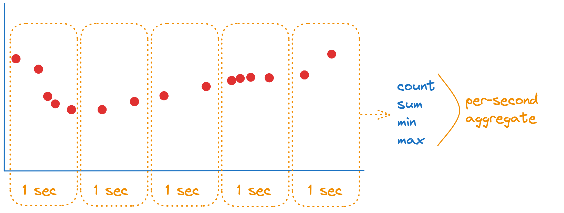
StatsHouse does not store an exact metric value per each moment. Instead, it stores aggregates associated with time intervals (see more about the minimal available aggregation interval).
Upon aggregation, StatsHouse inserts data into the ClickHouse database—specifically, into a per-second table. The amount of per-second data is huge, so StatsHouse downsamples data: per-second data is available for two days.
StatsHouse aggregates data within a minute and inserts it to a per-minute ClickHouse table. Similarly, StatsHouse aggregates per-minute data to per-hour one.
Minimal available aggregation interval
The currently available aggregate depends on the "age" of the data:
- per-second aggregated data is stored for the first two days,
- per-minute aggregated data is stored for a month,
- per-hour aggregated data is available forever (if not deleted manually).

Imagine a hypothetical product. For this product, we need to get the number of received packets per second. The packets may have different
- formats:
TL,JSON; - statuses: "correct" (
ok) or "incorrect" (error_too_short,error_too_long, etc.).
When the user-defined code receives a packet, it sends an event to StatsHouse, specifically, to an agent. For example, let this event have a JSON format and a "correct" status:
    {"metrics":[ {"name": "toy_packets_count",
     "tags":{"format": "JSON", "status": "ok"},
     "counter": 1}] }
Formats and statuses may vary for the packets:
    {"metrics":[ {"name": "toy_packets_count",
     "tags":{"format": "TL", "status": "error_too_short"},
     "counter": 1} ]}
Let's represent an event as a row in a conventional database. Upon per-second aggregation, we'll get the table below—for each tag value combination received, we get the row with the corresponding count:
| timestamp | metric | format | status | counter |
|---|---|---|---|---|
| 13:45:05 | toy_packets_count | JSON | ok | 100 |
| 13:45:05 | toy_packets_count | TL | ok | 200 |
| 13:45:05 | toy_packets_count | TL | error_too_short | 5 |
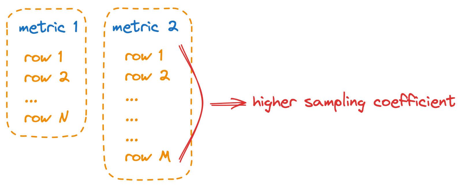
The number of rows in such a table is a metric's cardinality.
Cardinality
Cardinality is how many unique tag value combinations you send for a metric.
In the example above, the metric's cardinality for the current second is three as we have three tag value combinations.
The amount of inserted data does not depend on the number of events. It depends on the number of unique tag value combinations. StatsHouse "collapses" the rows with the same tag value combinations and summarizes the counters.
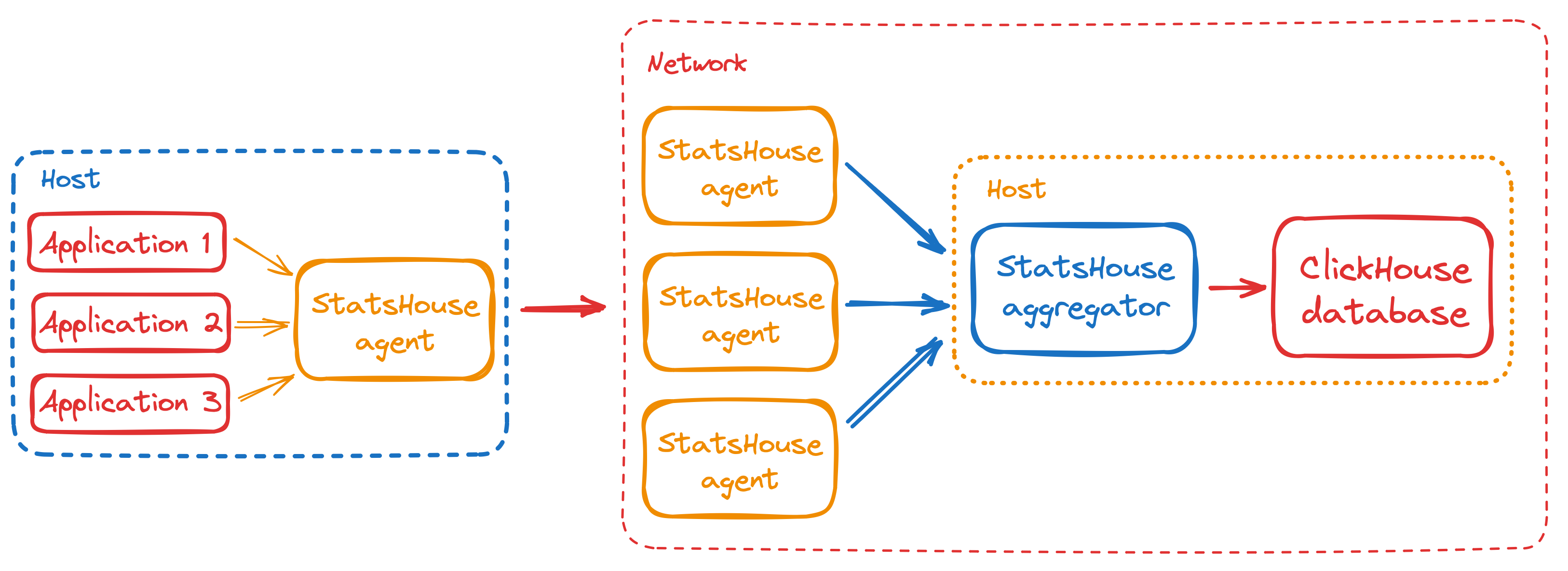
StatsHouse collects data from many hosts (agents) simultaneously. Upon collecting and aggregating data within a second, it sends data to aggregators.
For our hypothetical metric, the between-host aggregation per second leads to the following:
| timestamp | metric | format | status | counter |
|---|---|---|---|---|
| 13:45:05 | toy_packets_count | JSON | ok | 1100 |
| 13:45:05 | toy_packets_count | JSON | error_too_short | 40 |
| 13:45:05 | toy_packets_count | JSON | error_too_long | 20 |
| 13:45:05 | toy_packets_count | TL | ok | 30 |
| 13:45:05 | toy_packets_count | TL | error_too_short | 2400 |
| 13:45:05 | toy_packets_count | msgpack | ok | 1 |
Cardinality may increase due to between-host aggregation: the sets of tag value combinations for the hosts may vary. In the example above, the total cardinality for the current second is six.
The total hour cardinality for a metric determines how many rows for a metric can be stored in a database for a long time.
When retrieving data from a database, we have to iterate over the rows for the chosen time interval. It is the cardinality that determines the number of these rows and the time we spend on doing this.
Sampling
StatsHouse has two bottlenecks:
- sending data from agents to aggregators,
- inserting data into the ClickHouse database.

If the amount of sent or inserted data exceeded the aggregator's or database's capacity, it could lead to a processing delay. This delay could increase indefinitely or disappear if the amount of data was reduced. To ensure minimal delay, StatsHouse samples data.
Sampling means that StatsHouse throws away pieces of data to reduce its overall amount. To keep aggregates and statistics the same, StatsHouse multiplies the rest of data by a sampling coefficient.
Suppose we have three data rows per second for a single metric:
| timestamp | metric | format | status | counter |
|---|---|---|---|---|
| 13:45:05 | toy_packets_count | JSON | ok | 100 |
| 13:45:05 | toy_packets_count | TL | ok | 200 |
| 13:45:05 | toy_packets_count | TL | error_too_short | 5 |
Suppose also that the channel width allows us to send only two rows to the aggregator. StatsHouse will set
the sampling coefficient to 1.5, then randomize the rows, and send only the first two rows multiplied by 1.5.
The data sent will look like this:
| timestamp | metric | format | status | counter |
|---|---|---|---|---|
| 13:45:05 | toy_packets_count | TL | ok | 300 |
| 13:45:05 | toy_packets_count | JSON | ok | 150 |
or like this:
| timestamp | metric | format | status | counter |
|---|---|---|---|---|
| 13:45:05 | toy_packets_count | TL | ok | 300 |
| 13:45:05 | toy_packets_count | TL | error_too_short | 7.5 |
or like that:
| timestamp | metric | format | status | counter |
|---|---|---|---|---|
| 13:45:05 | toy_packets_count | TL | error_too_short | 7.5 |
| 13:45:05 | toy_packets_count | JSON | ok | 150 |
If each agent samples data in this way, it will throw away some rows. Upon aggregating data between the agents, the counters for the rows will be close to their original values (as if data was not sampled at all). The more agents aggregate their sampled data, the more accurate the resulting counters are.
The same is true for downsampling data: when StatsHouse aggregates 60-second rows to a one-minute row, or 60-minute rows—to a one-hour row.
The aggregates' averages will stay the same but will get the high-frequency noise.

We strongly recommend reducing metrics' cardinality.
The same algorithm applies both when the agents send data to the aggregator and when the aggregator inserts data into the database.
Non-integer sampling coefficients
Sampling coefficients should sometimes be non-integer to keep aggregates and statistics the same. This leads to non-integer values for counters, though each counter is an integer number at its core.
In StatsHouse, counters are floating-point by default.
For a particular metric, you can choose the option to randomly round the sampling coefficients:
if the desired sampling coefficient is 1.1, it will be rounded to 1 nine times out of ten—and it will be rounded to
2 only once.
Fair resource sharing
Now assume we have more than one metric, and they share the same channel of a given width. Ideally, the metrics should not affect each other. If a metric starts generating a lot more rows than the others, it should get the higher sampling coefficient, so that the other metrics are not affected.
The algorithm's logic is the following:
- StatsHouse sorts all the metrics in ascending order by a number of occupied bytes. Then it refers to them one by one.
- StatsHouse calculates the number of bytes to grant to each metric. The rest of the budget is shared between the rest of the metrics.
- If a metric does not spend its budget, its data is not sampled at all.
- If a metric exceeds its budget, StatsHouse samples it so that the metric data fits in the budget: for a metric with 2000 rows and the budget of 500 rows, the sampling coefficient is set to 4.
- StatsHouse reduces the rest of the budget by the number of bytes spent.
The number of occupied bytes depends on the metric type and the number of tag values. Counter metrics require less space than value metrics.
In practice, some metrics are more important than the other. StatsHouse administrators can set up weights for the particular metrics. A metric having a weight of 2 gets the channel two times as broad as the channel for a 1-weight metric.
Sampling "mainstays"
The above-mentioned algorithm works fine when the original counters for the rows are close to each other. Often, a metric has one or several "mainstays" that are dominating rows. For example, if we successfully process 1000 packets per second, but we also get one error of each type, the first "ok" row becomes the "mainstay":
| timestamp | metric | format | status | counter |
|---|---|---|---|---|
| 13:45:05 | toy_packets_count | JSON | ok | 1000 |
| 13:45:05 | toy_packets_count | TL | error_too_short | 1 |
| 13:45:05 | toy_packets_count | TL | error_too_long | 1 |
| 13:45:05 | toy_packets_count | TL | error_too_bad | 1 |
| 13:45:05 | toy_packets_count | TL | error_too_good | 1 |
When we display the sum of counters on a graph, we get the flat graph for the 1004 value.
Imagine, we have to insert only four rows out of five because of a budget. We will throw away one row per each second:
- for four seconds out of five the value will be
1003 * (5 / 4) ~ 1203, - for one second out of five the value will be
4 * (5 / 4) = 5.
On average, these values look valid: if we summarize them, we'll get 1004. But the graph will be located higher than
the average value—around 1200—and will have the ravines down to 0.
When StatsHouse has to sample such data (with "mainstays"), it divides the budget in two. The first part of the budget (two rows in our example) is granted for the non-sampled rows with the maximum counter values. The second part of the budget is spent for the rest of the rows: the random rows are inserted while the others are thrown away. Unlike "mainstays," these "weak" rows get the respectively higher sampling rate.
In our example, StatsHouse will insert the row with the 1000 counter as is, i.e., will not sample this row. So,
we'll get the graph with the average value of 1004.
User-guided sampling
Though it is better to let StatsHouse sample data for you, you may want to sample your data before sending them to StatsHouse. Use this kind of sampling to control the memory footprint.
In this case, you can explicitly specify counter for the value metric:
`{"metrics":[{"name":"my_metric","tags":{},"counter":6, "value":[1, 2, 3]}]}`
This means that the number of events is 6, and the values are sampled—as if the original value
was [1, 1, 2, 2, 3, 3]
Resolution
The highest available resolution of data to show on a graph depends on the currently available aggregate: you can get per-second data for the last two days, per-minute data for the last month, and you can get per-hour data for any period you want.
If getting the highest available resolution is not crucial for you, but it is important for you to reduce sampling, reduce your metric resolution.
For example, you may choose a custom resolution to make the agent send data once per five seconds instead of sending per-second data. StatsHouse will send data five times more rarely and grant five times more rows for the metric. The processing delay will increase by ten seconds:
- StatsHouse will be collecting data for five seconds,
- then it will shard data into five partitions,
- and will be sending data for the next five seconds—one shard per second.
This way of sending data ensures fair channel sharing for the metrics with differing resolution.
The resolution level may be a divisor of 60. To avoid jitter on a graph, use the "native" resolution levels: 1, 5, 15, 60 seconds. These levels correspond to levels of details (LOD) in the UI. If you choose a 2-second resolution level, the events will be distributed between 5-second LODs unevenly—two or three events per LOD:
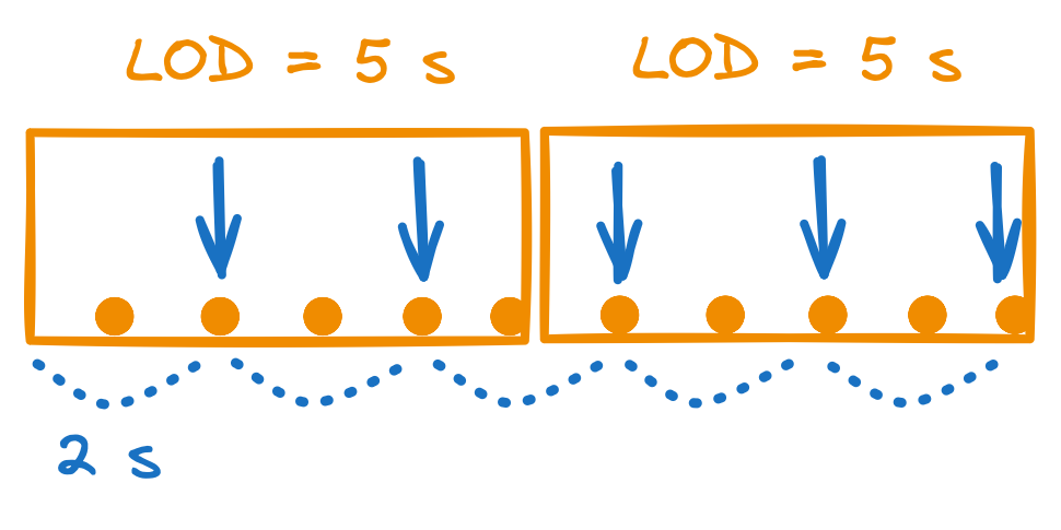
This uneven distribution leads to a jitter on a graph.